Fundamentals of reliable production scheduling.

Henri Muller.

Any manufacturer will have experienced the very irritating problems related to late delivery. Despite bulky inventories, every now and then a customer’s urgent need cannot be satisfied at the date agreed upon. The author shows the way out.

Goals and constraints.

Order-book and production schedule are the two aspects of one and the same reality. In the end, a new order coming in from any customer won’t be properly booked until it is inserted in a simulated production schedule. Depending largely on hazards of all kinds, the schedule must constantly be readjusted according to changes in the production conditions and to more or less important modifications in the customers’ orders. How, under such circumstances, can fairly reliable delivery dates be ascertained?

Processing is subject to three types of constraints:

·            capacities of the different production-units shaping the multi-processed products

·            minimal intervals between two operations (= processing steps)

·            prescribed product sequences at any production-unit for technical or economical reasons   

As a rule, new orders are registered at the half-empty end of the scheduled order-book, making use in the first place of the gaps left between previous insertions. Obviously, the product sequences at any of the processing units cannot obey sequencing constraints at the moment the orders are registered. Later on, order permutations will settle the question. A delivery margin, large enough to cover these permutations, will prevent late deliveries. Finally, the problem is solved by one single parameter per processing-unit: the permutation margin. The scheduled order-book will be a pre-schedule within which the final schedule with its permutations will be developed at the moment of processing.  

In order to get rid of any optimization procedures during pre-scheduling, the five targets aimed at are listed here below by decreasing priorities (occasional sequencing constraints will bring about larger inventories by grouping part of the orders for a smoother, cost-reduced processing; in this context, optimization becomes a necessity at the moment of ultimate scheduling):

(1):     respect the delivery terms agreed upon with the customers

(2):     offer to each customer the nearest possible delivery date

(3):     minimize inventories

(4):     maximize the load of the production facilities

(5):     minimize changes from schedule to schedule

Postponing delivery dates by adequate margins is the only way to get enough leeway for grouping orders, compensating production hazards, etc. An increase of inventory is the price to pay for it.

The second priority tends to maximize the loads of the different processing-units composing the plant; the customer, of course, is free to choose a later delivery date at his best convenience. The orders registered previously are liable to be moved back to earlier dates in order to make room for new orders. There again, for the sake of short delivery terms (and higher productions), inventories and their cost are on the increase. We assume that the additional production is profitable enough at least to take on these costs (thus escaping yet another optimization procedure).

Once the delivery date of an order has been fixed, the third priority tends to manufacture the order as near as possible to the agreed date (notwithstanding the fact that the order may finally be moved back to earlier dates).

The fifth priority brings in the current production schedule as a guide-line for updating the production process. The future schedule is derived from it by a strict application of the five priorities and their hierarchy while taking into account the changes that have meanwhile occurred in the order-book and on the shop-floor (breakdowns, advances, …). Continuity of scheduling is a necessity to put the customers’ minds at rest. By the way, it maintains the customers’ vested rights:

·            in opposition to the usual rule “first in, first out”, the agreed delivery date fixes the precedence of any order notwithstanding its entry-date (by preferring a postponed delivery date to the offered shortest possible one, the customer loses any priority over another man’s order to be delivered earlier than his, albeit it has been registered later than his)

·             the longer an order stays in the order-book, the more it runs the risk of being delayed by production hazards; however, compensations between ancient and recent orders will not take place 

Any pre-scheduling proceeds from four basic listings:

·            the inventories

·            the current production-schedule

·            the order-book

·            the characteristics of the batches

Basic notions.

An order coming in from the customer may concern different products. It is split up into batches of interchangeable items. For practical reasons, too big a batch may be broken up into a series of well-sized smaller ones.

The production facilities are assumed to be composed of any number of processing-units (production-units). According to its operational pattern, a given product passes (here in a sequence known beforehand) through some of the units, undergoing the planned operations. Depending on the product it belongs to, any item takes a specific processing-time per production-unit.

The capacity of any processing-unit depends on its time-schedule (the production a processing-unit is capable of depends on its time-schedule as well as on the mean processing-time of the product mix it has to work on).

Here, each unit being supposed to work round the clock, it can be represented by its time-axis, the origin (point zero) corresponding to the time of the day. After a breakdown or any interruption – scheduled or not, the origin of the processing-time of the concerned unit may happen to be postponed. Each point of any time-axis represents a date. The processing-time of a batch at a production-unit (belonging to its operational pattern) is the interval between its starting- and finishing-dates (at any unit the processing of any batch is not allowed to be interrupted on purpose).

Between two operations A and B following each other directly during the processing of one and the same batch at units F_A and F_B, there will be a time-gap, measured by the interval separating the finishing-dates (for instance) of operations A and B (cf. chart 1). Processing-time T_A of the batch may be longer or shorter than T_B. The gap is at least T_B – T_A (but cannot be inferior to zero). To this must be added the processing-time t_A taken in F_A by just one of the items composing the batch. Indeed, operation B cannot start until a first item has been delivered by F_A.

The transfer from unit to unit, as well as the conditioning of the products beyond processing-time (cooling, drying, fermenting,…) may sensibly increase the minimal gaps defined above. On top of it come the safety and sequencing margins that, in practice, are nothing but further extensions of the minimal gaps. By the shifting of the registered orders due to priority (2) the real gaps will in general exceed the minimal ones.

If the operational pattern is such as to process a given product repeatedly by the same production-unit, we must be able to handle loops. The gap between two operations X_n, X_n+1 carried out at the same unit F_X must at least be equal to the processing-time of the second operation X _n+1.

The operational processing-time and the gap between two of the operations carried out on one and the same batch are quite different notions. A tunnel-oven may have a very high output (the inverse of the very short mean processing-time = interval between two subsequent items leaving the furnace), while the unavailability of the products (= gap with respect to the previous operation) takes all the time – hours if not days – of their slow travel through the whole length of the oven and of their slow cooling in the open air. The processing-times concern the production-rates, the gaps concern the stay-times of the batches inside the production facilities.   

After each operation, during the time (of the gap) the batch is not available for further processing, it enters inventory. After each processing step, any operational pattern delivers a semi-finished product to the respective inventory. The pattern is thus shortened, leaving a stumped batch. The next operation must wait for the availability of the semi-finished product. The previous operation remains temporarily in the order-book as a ghost operation located at point zero of the concerned production-unit, its processing-time being reduced to zero, its minimal gap corresponding to the availability delay. Stumped batches are a quite normal consequence of the existence of operational patterns in multi-processing manufacturing.

Occasionally, as far as a processing-unit is fully loaded or scheduled for good, part of its load may be taken out of account. Point zero of the concerned unit is shifted accordingly; at this virtual origin virtual stumped batches will arise.

Tools.

A series of specific tools (= procedures) will greatly simplify the passage from order-book to schedule.

         Sequences.

We shall consider three kinds of sequences:

·            per batch, the sequence of operations that must be carried out (= operational pattern)

·            per processing-unit, the sequence of the batches as they have been scheduled so far (batch sequence)

·            for the whole of the production facility, the overall sequence of the batches each of them being represented by the starting-date of its very first operation 

         Up- and down-levelling.

The processing-times of two consecutive batches A, B that overlap at one and the same production-unit are separated by

·            shifting A back to earlier dates (= to the left) (up-levelling)

·            shifting B forward to later dates (to the right) (down-levelling)

The shifts change the gaps within the concerned operational patterns. If, for any batch A, the gap between the consecutive operations A_X and A_X+1 gets smaller than the minimum allowed:

·            A_X is shifted back to the left (up-levelling)

·            A_X+1 is shifted to the right (down-levelling)

This last shifting may jeopardize the result of the previous ones: the procedure gets iterative.

A down-levelling becomes necessary if the up-levelling results in negative starting-dates (below point zero). Before down-levelling at any unit concerned, the starting-date of the very first batch (of the batch sequence) will be shifted to the right until it coincides with point zero of the unit.

The levelling  doesn’t disturb the batch sequences.

         Load compression.

While maintaining the batch sequences of the moment at all processing-units, while keeping batches from overlapping and, inside the operational patterns, preventing gaps from getting undersized with respect to their minimal values, loads are as far as possible concentrated towards their zero points.

        Gap tightening.

The inventory potential of any load pattern concerns all the batches registered in the order-book. For each operational pattern, the potential is measured by the non weighted sum of all really existing gaps between operations, plus all advances of the final operations with respect to their delivery dates (late deliveries are neglected). In order to lower this potential, gaps above minimum value and advances are as far as possible shortened one by one. Any shortening is accepted if it neither increases the inventory potential nor causes or worsens late delivery of any batch. Moreover, the up-levelling consecutive to any shortening attempt is not allowed to result in negative starting-dates. If necessary, gap tightening alters the batch sequences.

Batch-insertion.

The comparison of loads, brute and compressed, reveals all insertion opportunities amidst the row of batches representing the load of the considered processing-unit. In chart 2,  the oblique lines point out, for each processing-unit, the space that can be made available between the starting-date of any batch (= operation in this case) and the finishing-date of the batch that immediately precedes it at the same unit.

For the insertion of a batch its operational pattern is split up into separate (partial) batches. These “batches” are independent except for the intervals between them that must not be inferior to the minimal gaps foreseen between the corresponding operations. The partial batches are numbered in the order of the operations they represent.

There are two modes of insertion:

·            the downstream mode: the partial batches are inserted one by one, starting with the first, ending with the last one; the insertion opportunities amidst the load are explored from the first up to the last of the already existing batches. The investigation starts at point zero of the considered processing-unit

·            the upstream mode: the partial batches are inserted one by one, starting with the last, ending with the first one; the insertion opportunities amidst the load are explored from the last down to the first of the already existing batches. The starting point of the upstream insertion is the most remote of two dates: either the shortest possible delivery date or the one agreed upon with the customer

In both instances, the investigation stops at the very first insertion opportunity.

After the insertion of each of the partial batches, levelling and compression must be resumed.

The insertion of a batch proceeds in three steps: 

(1):      downstream insertion in order to establish the nearest delivery date

(2):      upstream insertion (the downstream insertion having been undone) in order to reduce intervals (= inventory)

(3):      reassembling of the partial batches in order to form one single batch again

Up-dating the production schedule.

The procedure starts from the current production schedule.

To begin with, up-levelling will reveal all the irregular changes of the order-book as well as the short-comings of the shop-floor bringing about a series of negative starting-dates, i. e. late deliveries. In this case, a subsequent down-levelling will be necessary.

This having been done, the batches, following their overall sequence, are reinserted one by one. Each batch is at first put out of schedule (for the rest, at this stage, the schedule remains completely unchanged). Immediately, after being eliminated, the batch will be reinserted according to the procedures described above.

The reinsertion procedures may change the batch-sequences.           

Finally, gap tightening somewhat reduces the inventory potential of the load.

Application modes.

The method of insertion and up-dating by insertion may easily be adapted to processing conditions differing from those assumed here above:

·            to operational patterns having free sequences

·            to capacities varying in time

·            to multiple constraints coming on top of the global capacity limits

·            to linked processing-units

·            to composite production-lines working independently, their products being put together in assembly shops

·            to parallel processing-units

·            to production runs due to sequencing constraints

·            to preferential delivery dates

·            to split up capacities (production facility run jointly by different companies)

Charts.

Charts  2 to 5 refer to a production facility composed of 3 processing-units, loaded with 75 batches. The horizontal lines (one or two lines per unit) show the load of each of the three processing-units

Operational patterns limited to just one operation are coloured in red, green and blue; batches manufactured in two operations (independently of the prescribed sequences) are yellow, turquoise, lilac; three-operational batches (of different sequences) are shown in grey.

For each batch, delivery date, operational pattern, processing-times and minimal gaps have been determined by appropriate random generators.

The upper vertical lines mark the starting- and finishing-points of the batches.   

Chart 2 with its two horizontal lines for each processing-unit shows the real load (upper line) and the compressed one (lower line). The oblique lines correspond to the insertion opportunities.

The oblique lines of charts 3 and 5 link the operations undergone by each of the 75 batches.

Chart 3 represents the current schedule; charts 4 and 5 the way it has been adapted to breakdowns at the different processing units (chart 4: after up- and down-levelling; chart 5: after reinsertion and tightening).

With each chart, the lower diagram shows the divergence (advance, tardiness) between real and original delivery times.    

20-05-2006, 21:55 Geschreven door Henri  

20-05-2006, 21:54 Geschreven door Henri  

20-05-2006, 21:53 Geschreven door Henri  

20-05-2006, 21:53 Geschreven door Henri  

20-05-2006, 21:52 Geschreven door Henri  

20-05-2006, 21:52 Geschreven door Henri  

Targeting sales.

Henri Muller.

Keeping or extending market-shares, harmonizing markets and productions, maintaining the order-book at a convenient level and maximizing profits are the main, sometimes contradictory aims of the sales department. The department should have a precise knowledge of market developments, sales-prices, the company’s manufacturing capabilities and production costs. It requires the active help of the shop floor as well as of the book-keeping department. In the form of a synthesis this paper takes all relevant aspects into account and eventually yields a realistic and relatively simple computing method that could be very helpful to efficient salesmanship.

The bottom line of any company can be somewhat boosted by systematically pushing the sales of the most profitable products.

Two conditions must be fulfilled: there must be some excess of demand compared to the processing capabilities of the plant, lest there should be no possibility of choice left to the sales department; per product, the profitability must be known.

The most favorable quantity and price ranges of the different products and the different markets as assessed by the Commercial Department are on the one hand valuable information to the selling points all over the world, on the other hand a helpful clue to the salesman on the spot, facing his customer.

Despite its simplicity, the idea of selective sale must overcome some unexpected conceptual obstacles.

What are the potential markets open to given production facilities? The answer depends on the way the question is looked on:

· a market survey in many cases yields too large and too heterogeneous a demand: a vast range of specific needs at quite different price levels

· the immediate sales potential can be assessed by summing up the sales expectations for the current quarter of all the selling points

· a third method considers the existing product mix as it results from the sales carried out in the past. This mix is the outcome of years of selling practice and of matching demand and processing facilities as far as possible. Which however does not mean that it can’t possibly be improved at all (the starting mix of charts 1 to 5 will be fixed this way)

Operating by selective sales comes down to neglect the less profitable markets. The danger is that, once the relation with the customer has been broken up, it may be difficult to restore it afterwards, say in a period of recession. That’s why, even in less profitable areas, some level of activity is currently maintained, albeit with minimal quantities. Generally speaking, selective sales must compromise between profitability and customer diversity. Any increase in profit must be achieved with a minimal distortion of the demand.

Sales prices are fixed by the market. Reference prices, assessed by the Commercial Department, depend on the production mix which has actually been sold. The more selective the sales, the higher these prices. That is why the process of selection must be progressive. The mix has to be improved by small steps rather than abruptly, in order to avoid upsetting the relations with a large number of customers at short notice.

The reference prices of the products depend on their profit margins. Obviously, different products are to be compared exclusively by their variable costs. There is no sense in taking into account the fixed costs, because these, by their very definition, are independent of the mix. Furthermore, as anyway they cannot be correctly distributed among the different products, by attempting to do so one would unduly bias the results. Nevertheless, the production facilities, by matching mix variations, may imply some change in the fixed costs. Then, at the breaking point, appropriate scenarios, considering total costs (fixed and variables), will settle the question.

The notion of “bottleneck” is another delicate item. It cannot be denied that for a product undergoing different operations at different processing-units the delivery-date depends on only one of them. In complex production facilities the location of the bottleneck may change from product to product and, even, for one and the same product, from order to order. Generally speaking, as the future load of the facility is not known, the optimal mix is assessed by admitting the existence of more than one bottleneck at a time. As a matter of fact, each processing unit is a priori a potential bottleneck. Whatever the complexity of the facilities and the diversity of the products’ processing patterns, the computing procedures (quadratic programming) detect any unit that for a given mix is about to become a bottleneck (eventually, the said units reach more or less their saturation). Depending on incoming orders, some of the units – alternately – will really end up as bottlenecks. In a quite autonomous way, quadratic programming figures out the production-units that for a given product mix could happen to be filled up to their saturation point, as well as those whose capacity – in any event – will be in excess.

Four parameters are attached to each product:

v_i = selling price per quantity unit

k_i = variable production costs per quantity unit

m_i = vi – ki = brute margin per quantity unit

cr_i = production-time needed at production-unit r per quantity unit

The production costs k_i of product i are the sum of the costs – here the variable costs – occurring at all the production-units during the processing of the quantity unit of product i (in order to compensate any loss or gain of material during processing, the c_ri are assessed by measuring the quantities of product i processed at production-unit r in terms of finished product).

For each product there are two quantity variables:

q_i = demand (quantity per time-unit, per quarter, for instance)

p_i = production (quantity per time-unit, per quarter, for instance)

For one and the same product i quantities q_i, p_i are additive respectively.

Each processing-unit r has its capacity C_r (capacity = production-time available at production-unit r per time-unit, per quarter, for instance).

The “global” parameters are:

(1): P_r = Σ_i (p_{i *} c_ri) = total production-time necessary at production-unit r to process the whole of the production-mix scheduled for the quarter considered

(2): M = Σ_i (p_{i *} m_i) = total brute margin of the whole of the production scheduled for the quarter

Per product i the distortion (d_i) of the quarter is measured by the turnover (w_i = q_{i *} v_i) related to demand q_i, weighted by the square of the relative gap between the two turnovers, that of the demand (w_i = q_{i *} v_i) and that of the production (w_i = p_{i *} v_i): d_i = w_{i *} [(w_i – u_i ) / w_i)]² = w_{i *} (1 – u_i / w_i)².

The global distortion of the quarter amounts to

(3): D = Σ_i d_i = Σ_i [w_{i *} (1 – u_i / w_i)²] = Σ_i [q_{i *} v_{i *} (1 – p_i / q_i)²].

What exactly are the relations between demand, product-mix, distortion, production quantities, production capacities and margins?

The task of the Sales Department is a triple one: as far as possible satisfy the customers’ demand, keep the composition of the order-book abreast of the production possibilities, maximize the bottom-line.

As already pointed out, our approach makes sense only if the demand exceeds the production capabilities. Otherwise there would be no choice left and the mix would have to be accepted the way it’s coming in.

From a mathematical point of view, the second task is a constraint rather than an objective. As the location of the bottlenecks are not known beforehand, the constraints that limit the production are expressed by inequalities (P_r ≤ C_r). Other constraints concerning the production quantities come on top of it: in any case these quantities must not be inferior to zero; sometimes minimal quantities (p_i ≥ p_imin) are imposed. On the other hand, in many instances quantities must not exceed certain limits.

At this stage, we consider only two of the three targets, the conformity to demand being the main one. If temporarily the increase of benefits is completely neglected, the problem reduces to the minimization of distortion D, the limitation by the processing facilities and of the production quantities being taken into account. According to relation (3), D measures the gap between corresponding q_i’s and p_i’s.

If anyhow the capacity constraints keep the production from equaling demand, why not by the way boost certain products and thus increase general profitability? This must be done with the necessary care so as not to disturb too many customers at a time. As it is mathematically impossible to pursue simultaneously two different targets, the increase of profit is introduced in the form of a constraint (M according to relation (2)). The computation yields the minimal distortion D for a fixed brute margin M, which – inversely – comes down to fixing the highest possible margin for a given distortion.

An optimum of this sort (constrained optimum) is resolved by means of an auxiliary function F, where the constraints are weighted with respect to the main function D by the Lagrange multipliers L_r, L_i, L_M

(4): F = D + Σ_r [L_{r *} P_r] – Σ_i (L_{i *} p_i) – L_{M *} M

= Σ_i [q_{i *} v_{i *} (1 – p_i / q_i)²] + Σ_r [L_{r *} Σ_i (p_{i *} c_ri)] – Σ_i (L_{i *} p_i) – L_{M *} Σ_i (p_{i *} m_i)

(the expressions are preceded by + or – in a way conferring positive values to all the multipliers: D is to be minimized, M maximized, the P_r’s have upper, the p_i’s lower limits).

The F-function is minimized by the correct choice of the p_i’s. By nullifying the derivatives of F with respect to the p_i’s we get the algebraic expressions of the p_i’s (by means of e_i = ½ _* q_i / v_i)

(5): p_i = q_i + e_{i *} [L_{M *} m_i – Σ_r (L_{r *} c_ri) + L_i].

The problem of selective sales are thus completely solved by formulas (5) and the equalities and inequalities expressing the constraints

(6): Σ_i (p_{i *} c_ri) ≤ C_r, p_i ≥ p_imin, Σ_i (p_{i *} m_i) = M.

Due to the inequalities in (6), the problem, i. e. the assessment of the multipliers L_M, L_r, L_i and the p_i’s belongs typically to the realm of linear programming.

Parameters q_i, v_i (hence e_i), m_i, c_ri, C_r, p_imin are given. The imposed value of M evolves between its minimum value (point of zero distortion) and its utmost value (solution of pure linear programming regardless of distortion).

Expressions (3) and (1) allow to assess the degree of distortion (bare of any practical signification) and the load of the different production-units, independently of there being bottlenecks or not.

Starting with an existing mix, charts 1 and 3 show how the production-quantities of 35 products change with the increase of the total margin. The evolution of the total brute margin – given by [(M – M₀₀) / M₀₀] – brings about continuous changes of the mix – expressed by (p_i / q_0i) (M₀₀ et q_0i being the initial values of M and the q_i’s). The parameters of the products, more or less realistic, have been created by appropriate random generators.

Charts 1 and 3 give a general survey; for more detail charts 2 and 4 magnify the ordinate of charts 1 and 3 respectively. Charts 1 and 2 admit one single bottleneck. For charts 3 and 4 the five production-units occasionally form bottlenecks all at the same time.

The charts have been established by the “progressive method”: for each value of M the associated product mix becomes the demand of the next M-value. Any set of p_i’s converts at once into the q_i’s entering the computation of the set of p_i’s located at its immediate right (an infinitesimal progression dM of M – hence a continuous evolution of the q_i’s and p_i’s – would be ideal). It can be proven that the progressive method keeps the p_i’s from reaching values below zero. The p_i’s representing unfavorable products tend asymptotically towards nil. At the final point – the one of highest possible margin – the results of the quadratic and the pure linear programming are identical. There, the number of remaining products is equal to the number of remaining bottlenecks (not considering the products whose quantities have previously reached their imposed upper limit).

Reference prices.

According to relation (5), for increasing M, depending on the algebraic sign of expression [L_{M *} m_i – Σ_r (L_{r *} c_ri)], the p_i’s are growing or diminishing (for p_i’s not constrained by commercial limits the L_i’s are equal to zero). For each product i the difference between m_i and n_i = Σ_r [(L_r /L_M) _* c_ri] decides if, with respect to the prevailing mix and its mean brute margin, he product has to be pushed (m_i > n_i) or restricted (m_i < n_i). Adding the variable costs k_i to the brute reference margin n_i one gets the reference price s_i (= n_i + k_i) of product i.

But the resulting reference prices are biased. In the general case, ratios L_r / L_M have two components, the one related to the margin and the one related to distortion. Reference prices however must be bare of distortion elements. Now, the progressive method happens to change the L_r / L_M into the differentials a_r = dL_r/dL_M, which – as can easily be proved – are free of any trace of distortion. That is the decisive advantage of the progressive method and the reason to adopt it definitively. For production-unit r, a_r is the marginal value of its constraint C_r (the marginal value of a non bottleneck equals zero). Chart 5 shows the evolution of the a_r’s corresponding to charts 3 and 4.

The marginal values depend on the product mix and its profit potential. The a_r’s of production-unit r applies to all the products really or possibly processed by r. Their reference prices, at the point reached so far (i. e. for a given M), amount to n_i = Σ_r (a_{r *} c_ri) = a_{1 *} c_1i + a_{2 *} c_2i + a_{3 *} c_3i + a_{4 *} c_4i ... completed by the variable costs k_i of product i (the c_ri’s are supposed to be known, as well as the variable costs k_i; for any product not processed by r, c_ri equals zero). Any change of mix requires great care. Too brutal an additional sale of relatively important quantities of products, for the moment being of an apparent high profitability, may upset the bottleneck pattern to a point jeopardizing benefits.

Selective sales check the price structure rather than the price level. If for all products the selling prices equalled their references (v_i = s_i or m_i = n_i), mix variations wouldn’t have any effect, whatever the profitability of the sales. Start and end of any p_i-curve would coincide; there would be no curves at all. The general price level is a quite different, very important question, the one concerning the ratio between turnover and global production costs (fixed and variable).

In a large array of items, the introduction of distortion yields unexpected results in the following cases f. i: parallel production-units; search of a neutral (unbiased by profit boosting) load of the production-units for a given demand; homogenizing a set of different markets despite accepted price differences in order to compare the price structures from market to market in a way unbiased by these differences; assessment of selling prices outside and inside the company; spotting of the most harmful bottlenecks.

24-04-2006, 18:26 Geschreven door Henri  

L’échéancier fiable.

Fundamentals of reliable production scheduling.

Henri Muller.

Any manufacturer will have experienced the very irritating problems related to late delivery. Despite bulky inventories, every now and then a customer’s urgent need cannot be satisfied at the date agreed upon. The author shows the way out.

Tout entrepreneur sait à quel point il est difficile de respecter les délais de livraison accordés à une clientèle de plus en plus pointilleuse à cet égard. Trop souvent, la pléthore des stocks n’empêche pas les marchandises réclamées d’urgence de ne pas être disponibles à temps. On trouvera ici une analyse serrée des causes de telles défaillances et les remèdes à y apporter.              

Objectifs et contraintes. 

Echéancier et programme de mise en fabrication sont les deux aspects d’une même réalité. En dernier ressort, l’enregistrement de nouvelles commandes ne peut se faire qu’à partir de programmes de simulation. Dépendant dans une certaine mesure de facteurs aléatoires, l’évolution des productions doit constamment être réalignée sur l’échéancier, qui, à son tour, tient compte à tout moment des modifications imposés par les clients en ce qui concerne les dates précises de livraison, ainsi que les quantités et les produits mêmes à fournir. L’objectif de notre analyse est celle d’accorder en toute  circonstance des délais de livraison fiables, compatibles avec l’état du carnet des commandes et de l’outil de production. Inversement, les programmes de mise en fabrication doivent sans relâche être réactualisés.

La mise en fabrication est tributaire de trois types de contraintes techniques :

·            capacités de production des différentes installations et temps de production des produits)

·            durées d’élaboration des produits après mise en fabrication (déterminant la durée du séjour d’un produit dans la structure de production ; v. plu loin : coordination des opérations séquentielles sur un même article)

·            par installation, séquences prescrites ou préférentielles des différents articles à mettre en fabrication

En règle générale, les nouvelles commandes, fraîchement entrées, sont enregistrées dans la partie incomplète de l’échéancier, dans un environnement lacunaire. Voilà pourquoi, quand, à la mise en fabrication, l’ordre de succession des produits ou groupes de produits est prescrit (« prescriptions de séquence »), sauf cas particuliers, une simulation détaillée des productions ne sera possible que lorsque la charge complète des installations sera connue. En attendant, le problème peut être résolu par l’introduction d’un ou de plusieurs paramètres forfaitaires (« marges de séquençage »). Ils concrétisent la marge de manœuvre qui, lors de la programmation définitive, sera nécessaire à la permutation des commandes. La charge des installations ainsi établie servira de programme préliminaire dans lequel pourra s’inscrire la programmation finale

Rendant superflu le recours à des algorithmes explicites d’optimalisation, la hiérarchisation univoque des priorités mène, par définition, à des résultats optimaux (les algorithmes d’optimalisation ne sont d’application qu’a posteriori dans le cas de séquences prescrites ; ils cherchent à établir, lors de la programmation finale, l’équilibre le plus avantageux entre frais de stockage et coût de mise en œuvre du programme):

(1):      respecter les échéances convenues

(2):      offrir à la clientèle les échéances les plus rapprochées possibles

(3):      minimiser les stocks finals et intermédiaires

(4):      maximiser les charges des installations

(5):      maintenir dans la mesure du possible la continuité de la programmation

Les marges tampon inclues forfaitairement dans les délais de livraison limitent les risques de dépassement des dates de fourniture. Généralement la détermination de ces marges est empirique.

La deuxième priorité tend à densifier autant que possible la charge des installations. Le client est libre néanmoins de choisir une date de livraison ultérieure quelconque, convenant le mieux à ses besoins. Les lots déjà en place sont susceptibles d’être avancés afin de libérer les capacités nécessaires à la réalisation des nouveaux lots aux dates voulues. Le procédé, qui a l’avantage de compacter les charges, a l’inconvénient de majorer les stocks. Normalement, on devrait être en droit d’admettre que la profitabilité de l’entreprise permet au supplément du chiffre d’affaires de couvrir au moins les frais de production et de stockage qu’il implique.

Une fois l’échéance fixée, la troisième priorité fait réaliser le lot le plus près possible de sa date de livraison. Les stocks s’en trouvent diminués. Les charges ainsi libérées augmentent les chances des nouvelles commandes de se faire livrer dans les délais les plus brefs.

C’est la cinquième priorité qui oblige à fonder l’actualisation des charges sur le programme de production en cours. La mise en conformité avec l’échéancier se fait en suivant strictement les priorités (et leur hiérarchie) énoncées ci-dessus, tout en s’écartant le moins possible du programme tel qu’il se présente à ce moment-là. La continuité de la programmation rassure les clients et, de surcroît, sauvegarde leurs droits acquis :

·            à l’opposé du principe « premier entré – premier servi », ce sont leurs dates de livraison convenues et non leurs dates d’enregistrement qui décident des préséances des différentes commandes. En imposant une date ultérieure à la date la plus rapprochée possible, le client renonce à toute priorité par rapport aux commandes à dates de livraison antérieures, même si elles ont été enregistrées après sa commande à lui

·            une commande risque d’autant plus des retards pour causes de d’interruptions non voulues de la production que son séjour dans le carnet est long ; cependant, une égalisation des retards entre commandes nouvelles et anciennes n’aura pas lieu

Compte tenu des cinq priorités, toute programmation se fonde sur trois relevés :

·            caractéristiques des lots (par lot : nombre, types, suite et durées des opérations à subir ; durée minimales entre opérations) 

·            l’échéancier 

·            par installation, séquences de mise en fabrication prévues au programme en cours.

Notions de base.

Les commandes émanant des clients et comportant des produits différents sont subdivisées en références (rubriques, lignes), dont chacune correspond à des articles strictement interchangeables.  Pour des raisons de convenance, à l’occasion, les références peuvent être scindées en lots (batches).

Un nombre quelconque des installations faisant partie de la structure (du réseau) de production fait subir aux articles chacune une transformation (opération) spécifique (ici dans un ordre  prédéterminé). En principe, à travers le réseau de fabrication, chacun des articles suit son parcours propre ; l’ensemble des opérations auxquelles il est soumis représente sa gamme opératoire (operational pattern). Par installation, chaque produit est transformé à une cadence qui lui est propre (inverse du temps de production nécessaire à la réalisation d’un article, ici constant dans le temps et indépendant de la suite des articles à l’installation considérée).

La capacité de production d’une installation dépend de son calendrier de travail.

Ici, dans l’hypothèse d’une disponibilité continue de toutes les installations, chacune d’entre elles est représentée par son axe des temps, ayant la date du jour comme point zéro. Suite à une panne, par exemple, le point zéro de l’installation considérée peut ne pas coïncider avec la date du jour.    

Sur l’axe des temps, chaque point représente une date. Le temps de production d’un des lots à une des installations faisant partie de sa gamme opératoire est le laps de temps s’écoulant entre ses dates de lancement et de réalisation (une interruption intentionnelle de la transformation en cours n’est pas admise). Par installation, le passage des lots ne peut être que séquentiel.

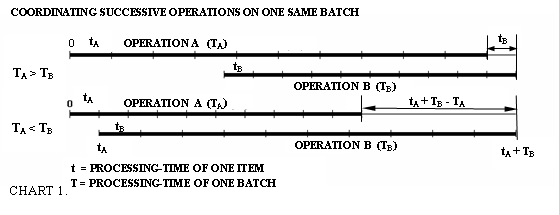
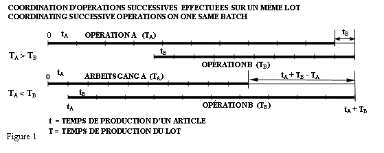
L’écart entre deux opérations A et B immédiatement consécutives effectuées sur un même lot par les deux installations F_A et F_B est mesuré par le laps de temps séparant les dates de réalisation de A et de B. Le temps de production du lot, T_A, peut être supérieur ou inférieur à T_B. L’écart doit être au moins égal à  T_B – T_A, sans cependant pouvoir devenir plus petit que zéro (v. figure 1). Vient s’y ajouter le temps de production t_A d’un article en A car l’opération B ne peut démarrer avant que le premier article en provenance de B lui soit parvenu. Les temps de transfert d’installation en installation et le conditionnement des produits (imposés par les procédés de fabrication : refroidissement, séchage, fermentation, …) peuvent accroître l’écart minimum. En outre, pour des raisons de sécurité, cet écart est à l’occasion prolongé dans le but de créer, tels que prévus, les stocks tampon intermédiaires ou finals. En cas de prescriptions de séquence, la marge de manœuvre pour permutations a posteriori vient encore gonfler les écarts entre opérations (p. ex., un produit réalisé une fois toutes les trois semaines par une campagne de production de 5 heures demande une marge de séquençage de 1.5 semaines). L’ensemble de ces écarts entre opérations immédiatement consécutives effectuées sur un même lot sera désigné par « décalage chronologique ». Il s’agit d’un minimum que, sous peine de retards, l’écart effectif doit au moins égaler, mais auquel, par les nécessités de la programmation (notamment du fait de la priorité (2)) il arrive d’être dépassé.

Si la gamme opératoire fait passer le lot directement (ou après un détour par d’autres installations) une deuxième, troisième, … fois par une même installation F_X, nous sommes en présence de boucles. Le décalage chronologique de base entre les opérations successives X_n, X_n+1 constituant une boucle doit être égal ou supérieur au temps de production en X_n+1 ; sinon, le décalage doit être majoré en conséquence (le décalage de base est la somme des décalages minimaux – déterminés en l’absence de boucles – propres aux opérations situées entre X_n,et X_n+1,  celui de X_n+1)y inclus).

Après avoir subi une des opérations, le lot n’étant pas immédiatement disponible pour sa transformation subséquente, il est mis en stock. pendant un temps égal à son décalage chronologique. Durée de non disponibilité ou délai de disponibilité (décalage chronologique par rapport à l’opération immédiatement précédente) et temps de production (durée d’exécution  de l’opération considérée) sont des grandeurs fondamentalement différentes. Pour les fours tunnels à forte production, que les produits traversent à faible vitesse avant de subir un refroidissement de longue durée, la différence est particulièrement prononcée. Le débit (inverse du temps de production) se mesure en secondes ; la traversée du four et le refroidissement des produits – la durée d’élaboration – prennent des heures, sinon des jours.

En plus des caractéristiques des produits, de l’échéancier et de la succession des lots au programme de mise en fabrication du moment, la gestion du carnet est fondée sur le relevé des stocks.

Toute gamme opératoire en cours d’exécution mène à chacune des étapes de sa réalisation à la mise en stock du demi-produit correspondant. La gamme s’en trouve raccourcie : il y a naissance d’un lot tronqué. Comme la transformation consécutive du lot concerné ne peut se faire avant sa date de disponibilité, l’opération la dernière effectuée reste conservée en tant qu’opération fantôme, se situant au point zéro de l’installation afférente, ayant un temps de production réduit à zéro et un décalage chronologique égal au solde du délai de disponibilité. La création de lots tronqués n’est pas un phénomène exceptionnel ; elle est continue en tant que conséquence normale d’une production par gammes opératoires.

À l’occasion, la partie saturée ou définitivement programmée des installations peut être mise hors programme moyennant une translation correspondante des points zéro ; à l’endroit des points zéro virtuels naîtront des lots tronqués virtuels.

Après leur expédition, les lots quittent l’échéancier. Par lot, échéance et date d’expédition coïncident. En principe, l’échéancier fait également fonction de plan d’expédition. Abstraction faite de cas de force majeure, les dates d’expédition convenues avec les clients lient les deux parties.

Outils.

Pour commencer, nous allons créer les outils nécessaires à l’actualisation des charges.

Séquençages.

Il faut distinguer trois sortes de séquences (de suites) :

·            par lot, la suite des transformations que subissent les lots du fait de leurs gammes opératoires respectives (suite des opérations) ;

·            par unité de production, la suite des lots et notamment celle de leurs dates de réalisation ;

·            pour l’ensemble des installations, la suite des commandes et notamment celle des dates de lancement des toutes premières transformations qui correspondent à leurs gammes opératoires respectives.

Lissages descendant ou ascendant (down-, up-levelling).

Tous les lots A, B, qui à une même unité de production se chevauchent plutôt que de se suivre conformément à une séquence donnée sont départagés en faisant

·            soit avancer A jusqu’à faire coïncider sa date de réalisation avec la date de lancement de B (lissage descendant),

·            soit reculer B jusqu’à faire coïncider sa date de lancement avec la date de réalisation de A (lissage ascendant). 

Ces déplacements font varier les écarts au sein des gammes opératoires. Si, pour un lot quelconque A, l’écart entre deux opérations consécutives A_x et A_x+1 en devient inférieur au décalage chronologique (minimum admissible), il y est ramené en faisant

·            soit avancer l’opération d’amont A_x (en cas de lissage descendant),

·            soit reculer l’opération d’aval A_x+1 (en cas de lissage ascendant).

Suppression des chevauchements et rétablissement des écarts pouvant se contrarier, les procédures de lissage sont itératives.

Le lissage ascendant n’est effectué que si le lissage descendant a abouti à des dates de lancement inférieures au point zéro de l’une ou de l’autre unité de production. A chacune des unités concernées, la date de lancement du premier lot de la séquence est alors alignée sur le point zéro correspondant.

Les lissages laissent inchangé l’ordre de succession des lots.

Compression des charges.

En maintenant les séquences (suites des lots), en évitant tout chevauchement de lots et en respectant les écarts minimaux entre opérations, les charges sont refoulées autant que possible vers les points zéro des différentes unités. 

Resserrement des écarts.

Le « potentiel de stock » d’un schéma de charge donné concerne tous les lots qui y figurent et notamment leurs gammes opératoires. Il est la somme non pondérée de tous les écarts effectifs entre opérations, auxquels viennent s’ajouter les avances des dates de mise à disposition finale par rapport aux échéances correspondantes (les retards n’étant pas mis en compte).

Dans le but de réduire ce potentiel, écarts et avances sont dans la mesure du possible ramenés un à un à leurs valeurs minimales. Tout resserrement est acceptable pour autant qu’il ne fait pas augmenter le potentiel de stock et ne met pas en retard un quelconque des lots par rapport à son échéance ou n’accentue pas un retard préexistant (le lissage descendant qui suit toute tentative de resserrement ne doit pas mener à des dates de production inférieures aux points zéro).

Insertion d’un lot.

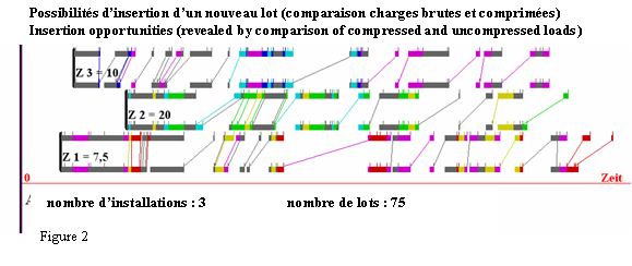
En comparant charges brute et compactée d’une installation, toutes les possibilités d’insertion quant à la taille et au délai de livraison du lot se révèlent. Au diagramme 2, les traits obliques indiquent par installation l’espace disponible entre la date brute de lancement d’une opération quelconque et la date compactée de réalisation de l’opération qui la précède immédiatement.

L’insertion d’un lot se fait séparément pour chacune des opérations faisant partie de sa gamme et ce en trois étapes, dont les deux premières, en tenant compte des décalages chronologiques entre opérations d’une installation à l’autre, profitent systématiquement des premières occasions d’insertion :

·            d’abord, afin de déterminer la date de livraison minimale, insertion d’amont en aval, de la première à la dernière opération du lot à insérer

·            ensuite, afin de minimiser les écarts entre les opérations, insertion d’aval en amont, de la dernière à la première des opérations du lot à insérer ; la deuxième étape a comme point de départ, soit la date de livraison minimale, soit une date de livraison ultérieure, demandée par le client

·            finalement, formation d’un seul lot à partir des opérations insérées séparément    

Après l’insertion de chacune des opérations, lissage descendant et re-compactage de l’ensemble des charges s’imposent. 

Actualisation du schéma de charge.

La charge qui correspond au programme en cours est le point de départ des procédures.

On tient compte des changements de programme non réglementaires en effectuant d’abord un lissage descendant. Si, à une installation quelconque, la date de lancement de l’un ou l’autre lot s’en retrouvera inférieure au point zéro afférent, un lissage ascendant s’en suivra.

Dans un ordre correspondant à la suite des commandes, chaque lot, en évitant de déplacer un quelconque autre lot, est d’abord éliminé des charges pour, à l’instar d’un lot fraîchement entré, être aussitôt réinséré (comme ci-dessus en trois étapes). En cas de livraison tardive, en deuxième étape, le  point de départ de l’insertion sera le résultat de la première étape ; dans le cas contraire, on partira de l’échéance (à la réinsertion, certains autres lots seront avancés). 

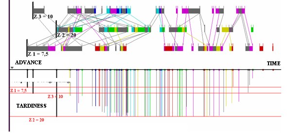
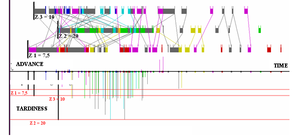
Les figures 4 et 5 montrent comment, en cas d’avance aussi bien que de retard, l’actualisation des charges, compte tenu des circonstances du moment, détecte les positions optimales des lots et de leurs gammes opératoires respectives.

Finalement, la procédure de resserrement des écarts est à même de réduire quelque peu le potentiel de stock du schéma des charges.

Applications diverses de l’algorithme de pré-programmation.

La méthode s’adapte aisément à des conditions de production autres que celles traitées ci-dessus[1] :

·            à des gammes opératoires dont l’ordre des opérations peut être quelconque

·            à des capacités fonction du temps calendaire

·            à des contraintes multiples s’ajoutant aux simples contraintes de capacité globales

·            à des installations couplées

·            à des produits composés, dont les éléments sont élaborés dans des ateliers spécialisés, chacun aux gammes opératoires quelconques, pour être assemblés dans des ateliers de montage intermédiaires et finals

·            à des installations parallèles (avec allocation optimale des produits)

·            à des campagnes de production (production runs)    

·            à l’attribution d’échéances de faveur

·            à la partition des capacités en cas de filiale exploitée en commun par plusieurs entreprises distinctes

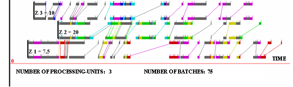
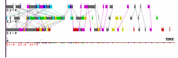
Les figures 2 à 5 se rapportent à une structure de production à 3 installations avec une charge de 75 lots. Elles visualisent par des barres horizontales (une ou deux barres par installation) les charges respectives des 3 installations.

Les lots rouges, verts ou bleus sont réalisés chacun en une seule opération aux installations 1, 2 et 3 respectivement ; les lots jaunes, turquoises et lilas sont réalisés dans l’un ou l’autre ordre (prescrit) aux installations 1, 2, 3 respectivement ; les lots réalisés en trois opérations, quel qu’en soit l’ordre de succession (prescrit), sont de couleur grise. Par lot, les dates de livraison, les gammes opératoires, les temps de production et les décalages chronologiques ont été fixés à l’aide de générateurs de hasard.

Les traits verticaux supérieurs représentent limites entre lots.

La figure 2 est la seule à avoir deux barres par installation, les barres supérieures représentant les charges effectives, les inférieures les charges compactées. Les traits obliques correspondent aux possibilités d’insertion aux différentes installations.

Les traits obliques des figures 3 à 5 relient les opérations subies par un même lot.

En raison de pannes, aux figures 4 et 5, les points zéro (Z₁, Z₂, Z₃) des installations sont décalés de 7.5, 20 et 10 unité de temps respectivement par rapport à la date du jour (une unité de temps correspond à la durée moyenne des opérations).

Par lot, les diagrammes aux barres verticales (au bas des figures) indiquent l’avance (réalisation prématurée : barres dirigées vers le haut) ou le retard (réalisation tardive : barres dirigées vers le bas) de la dernière opération par rapport à son échéance (compte tenu de la durée d’indisponibilité avant expédition).

08-12-2005, 20:49 Geschreven door Henri  

08-12-2005, 20:40 Geschreven door Henri  

08-12-2005, 20:39 Geschreven door Henri